Simulating Metal Prices - Copper
July 12, 2021
I am not a mineral economist or a commodity specialist. This goes for most of us in the Mining Industry. Nevertheless, we all need an appreciation for how mining projects and operations will react to changing commodity prices or, better still, the probabilities of seeing those commodity prices that trigger profound reactions. This need goes beyond the typical practice of assuming a short, medium and long term price and arbitrarily selecting sensitivity factors.
What would be really useful is a stochastic approach rooted in historical observation. Such an approach would allow us to say things like “The odds of the mine going on care and maintenance in its current configuration over the next three years are 20%” or “There are even odds that an expansion in production will create windfall profits within the next five years.” To pull this off, we need the ability to simulate future commodity price paths that are realistic.
My uncertainty about the future copper price is high. Again, not being a commodity specialist, the fundamentals of the copper market escape me. I have this fuzzy idea of how knowledge of changing demand, existing inventory, new production and mine shut-downs provide information today about prices tomorrow. However, I have not put in the time and effort to develop this knowledge. For me, the market fundamentals are unknown and my level of uncertainty remains high. However, it is not infinitely high. If I make the subjective call that future price movements will mirror the past, I can resort to some technical analysis to sweep away large portions of uncertainty.
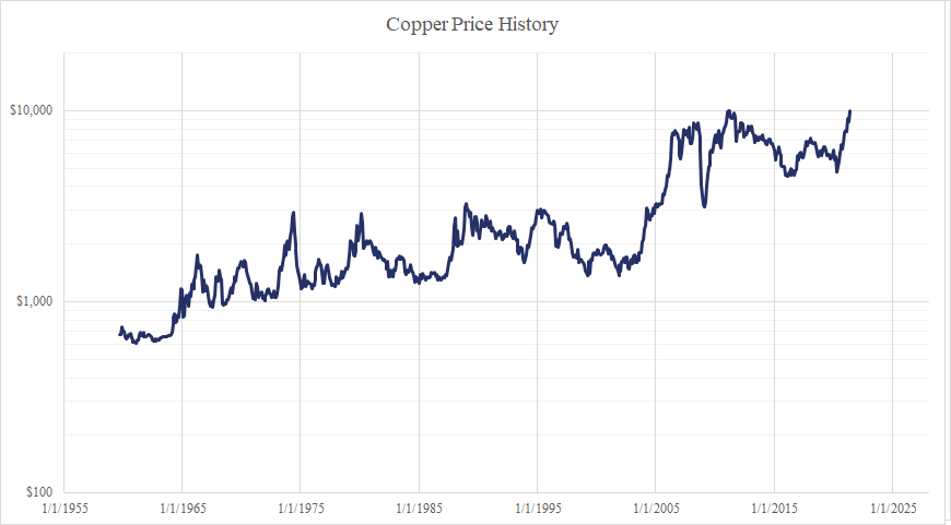
To proceed, I need to describe the statistical properties of past price movements. The chart below shows some copper price history data (monthly) I pulled from investing.com. From August 1959 through May 2021, the copper price has spanned the range of $1k to $10k per metric tonne and has arguably undergone exponential growth.
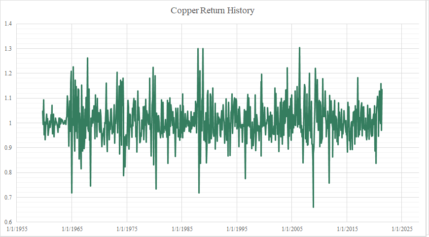
For now, I do not want to work with raw prices due to high autocorrelation where almost everything I need to know about today’s price is given in yesterday’s price. To eliminate this, I focus on copper price returns. Here I’ll define returns as the price of copper in a given month divided by the previous month’s price. The next chart shows the monthly copper returns for the past 62 years. The high autocorrelation we saw in the raw price history is eliminated. With this perspective, I interpret the first property of historical copper returns: returns are drawn from a random variable that is uncorrelated with the past.
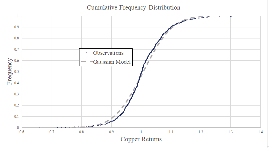
The next step is to define a model for the distribution of returns. The natural, but ultimately unsatisfactory, starting point is to calculate the mean and standard deviation of the observed returns and assume a Gaussian (Normal) Distribution. The chart below compares such a model to the observations, indicating a poor fit. Of particular concern are the tails. The observations are more fat-tailed than the Gaussian model, implying that, historically, extreme returns are more frequent than modeled. To overcome this, I built a more complicated model to fit the data, involving a Gaussian Distribution for the middle of the population and two Pareto Distributions to describe the left and right tails.This model distribution represents the second property of historical copper returns. Together the two properties define what I am willing to call realistic price movements.
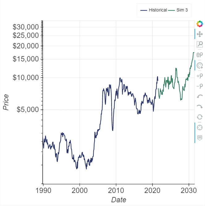
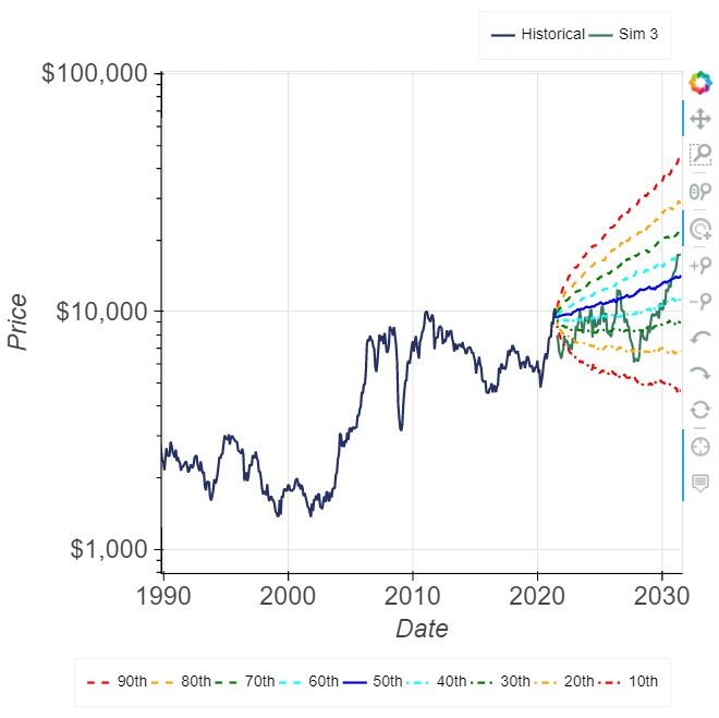
All that is left to do is simulate future price paths for copper that mirror these two properties. For a single price path we first need to acquire the current copper price, which, as of writing, is US$9,538 per metric tonne. To simulate next month’s price, I pull a random value from my model return distribution. I just did it and got 1.04. This multiplied by last month’s price gets me this month’s simulated copper price of US$9,920. This price multiplied by another random draw from my model return distribution simulates the following month’s price, and so on for as many months as I want. This chart shows the last three decades of copper prices and a single simulated price path for the next decade.
Repeating this process one thousand times yields one thousand price paths, each of which I interpret to be equiprobable. It would be a complete mess to plot all of these up on the same chart. A clearer presentation is to plot the percentiles as done below. The percentile lines allow me to see what percentage of the simulated prices paths fall below a given price in a given month in the future.
For those willing to register and login to my site, I have provided a tool (click here) for exploring these simulated price paths over the next decade. Along with copper, this tool includes gold, silver and nine other commodities (all properly correlated with each other). For those interested in a higher level of service, I can also provide an Excel file with all simulations that are easy to integrate into a cash flow model. Contact me for details.